 Nabil OMRI
- Posted on
Generating accurate and explainable predictions is truly amazing, isn’t it ?

Have you ever wondered how artificial intelligence (AI) systems make decisions? In the world of AI, there is a growing focus on developing models that not only generate accurate predictions but also provide explanations for their outputs. This concept is known as explainable AI, and its importance cannot be overstated. Let’s take a moment to discuss why explainable AI matters.
Transparency and understandability are key aspects of any AI system. When an AI model can explain the reasoning behind its decisions, it instills a sense of trust and accountability. Imagine relying on an AI-powered medical diagnosis tool. You would want to understand why the system arrived at a particular diagnosis. Thus, explainability is not just a luxury but a necessity since it empowers users to validate and interpret the outcomes produced by AI models, allows them to identify potential biases or errors and provides an opportunity for course correction.
In this context, several explanation techniques have been proposed. These techniques can be categorized into two main groups:
- Transparent models: These models exhibit an inherently explainable behavior. Examples include Decision Trees, Logistic Regression, and other interpretable models.
- Post-Hoc techniques: These techniques serve as interpreters applied to complex models to explain their behavior. Examples include LIME, Anchors, etc.
This article focuses on the group of transparent models, specifically highlighting a recently introduced technique called “Cyclic Boosting”. This technique emerged in 2021 through the work of a German research group.
The Cyclic Boosting is a new machine learning algorithm that guarantees high performance while also allowing for a precise understanding of the path taken for individual predictions. It can be used in three scenarios: multiplicative regression mode Y ∈ [0, ∞), additive regression mode Y ∈ (−∞, ∞), and classification mode Y ∈ [0, 1]. The predicted values of the target variable, denoted by y_hatᵢ , are calculated from given observations xᵢ of a set of feature variables X in the following way:

where fᵏⱼ represent the model’s parameters associated with each feature j and bin k. Here, categorical features maintain their original categories, while continuous features are transformed into discrete bins with either equal widths or the same number of observations.
To gain a deeper understanding of the mathematical formulation of the Cyclic Boosting algorithm, it is beneficial to utilize a specific example that will be employed subsequently to illustrate the underlying principle of this technique. Let us consider “item_X”, a product for which we aim to predict future sales based on seasonal variations.
| Season | Sales |
| Spring | 10 |
| Summer | 5 |
| Autumn | 12 |
| Winter | 20 |
| Spring | 9 |
| Summer | 7 |
| Autumn | 15 |
| Winter | 18 |
In this scenario, the feature number, denoted as p, is set to 1, indicating a single feature being considered. Additionally, the number of bins, denoted as K, is set to 4, representing the seasons (Spring, Summer, Autumn, and Winter). Consequently, the model’s parameters are calculated based on the training data using the following meta-algorithm:
- Calculate the global average µ from all observed y across all bins k and features j: μ = 12
- Initialize the factors fᵏⱼ(t=0) ← 1
- Cyclically iterate through features j = 1, …, p and calculate in turn for each bin k the partial factors g and corresponding aggregated factors f, where indices t refers to iterations of full feature cycles as the training of the algorithm progresses:

I understand that mathematical calculations can be challenging to comprehend. However, let’s simplify it using our example:
- g(t=1){Spring} = (10+9)/(12+12)=19/24 where the estimated output is calculated from the first formula where f(t=0) is set to 1. Then, f(t=1){Spring} = 19/24
- g(t=1){Summer} = (5+7)/(12+12) = 1/2 , and f(t=1){Summer} = 1/2. In the same way: f(t=1){Autumn} = 27/24 , and f(t=1){Winter} = 38/24
4. This process is repeated for t = 1, …, n until specific stopping criteria are met. These criteria may include reaching the maximum number of iterations or observing no further improvement in an error metric, such as the mean absolute deviation (MAD) or mean squared error (MSE).
This example illustrates the functioning principle of the Cyclic Boosting algorithm for a regression problem. For binary classification, the principle remains the same with a small modification in the target variable. In fact, the target variable range of [0, 1] represents the probability pi of belonging to the class or not. Thus, the odds ratio pᵢ /1 — pᵢ within the range [0, ∞] can be used as target variable following an approach similar to multiplicative regression:

Now, it’s time to start coding !
First, install the cyclic-boosting package and its dependencies
pip install cyclic-boostingThe model is implemented as a scikit-learn pipeline, stitching together a Binner and the cyclic-boosting classifier estimator.
from cyclic_boosting.pipelines import pipeline_CBClassifier
CB_clf = pipeline_CBClassifier()
CB_clf.fit(X_train, y)
y_pred = CB_clf.predict(X_test)
For more details, a complete regression and classification examples of codes are available here.
To assess its explanatory power, the Cyclic Boosting algorithm is applied to a modified version of the Titanic dataset. This application aims to predict the likelihood of survival based on the passenger’s ticket class, gender, and age. Once the model is trained, it can be evaluated by computing various metrics, including the mean absolute deviation or the scikit-learn in-sample score:
mad = np.nanmean(np.abs(y - yhat[:, 0]))
in_sample_score = CB_est.score(X, y)
Regarding the explanation functionality, Cyclic Boosting provides numerous informative training reports. These reports can be summarized and generated as a PDF using the following code:
def plot_CB(filename, plobs, binner):
    for i, p in enumerate(plobs):
        plot_analysis(plot_observer=p, file_obj=filename + "_{}".format(i), use_tightlayout=False, binners=[binner])

plot_CB("analysis_CB_iterlast", [CB_est[-1].observers[-1]], CB_est[-2])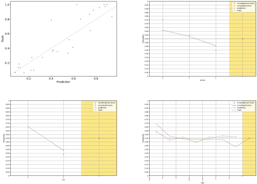
According to the obtained results :
- Female passengers have the highest likelihood of survival,
- Passengers in the first and second classes have significantly better chances of survival.
- Age is generally not a crucial factor, it becomes more significant for younger individuals (age < 18 years) who have a higher probability of surviving.
Additional examples of plots and their interpretations can be found in the Cyclic Boosting documentation.
For more details about the Cyclic Boosting algorithm, you can refers to the following materials: